Exercise 6 - Exploring the Stroop adjustment data
Contents
Exercise 6 - Exploring the Stroop adjustment data#
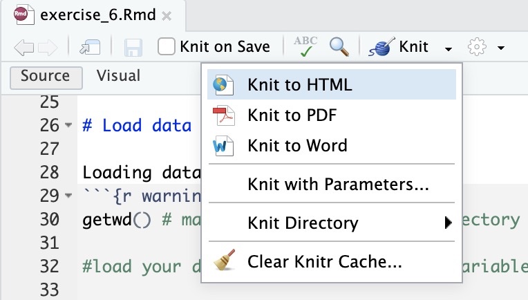
Because you’ll submitting a continuous notebook (rather than developing a program) for this exercise, there’s no need to have multiple tags. I encourage you though to make regular commits as you’re working on the assignment. The final commit should be tagged Exercise_6_done and have a single notebook called exercise_6.Rmd that has clearly titled chunks (see starter code). Insert additional chunks as you see fit. Make sure you push all the files in your working directory to the repository, not just the Rmd file. This will help us run your code. To help us grade quickly, make sure to also include a knitted .html file.

Important
Open your notebook using the included .Rproj file. If you don’t, you’ll likely be in the wrong working directory and will have trouble loading the data using the starter code.
Part 1#
Inside the data subfolder are individual data files. Each file has a column header and is comma-delimitted. We need to read them into a single R dataframe (dat). The starter code provides a way for you to read all these files into a single R data-frame. I would also like you to practice doing this by concatenating all the files in your shell. See here for how to concatenate multiple files into one (the only slightly tricky part is what to do about the column headers).
Note
R has (too!) many functions for reading in CSV files. Some of them are much slower than others and should be avoided if you’re reading in lots of large files. See here for a discussion and time comparison of the different functions. Different functions also have different column-type defaults (e.g., reading in a column containing text-strings as factors vs. character vectors).
To show that you’ve understood how to do file concatenation in the shell, please add in the commands you used in the indicated place in the R notebook and write an aggregated_data.csv file into a aggregated_data directory that contains the output of your shell command(s). This file should be pushed along with the rest of your submission.
Part 2#
Compute correct RTs only
Whenever we look at RTs, we don’t want to mix together RTs from correct and incorrect responses. Subset your data-frame to include only the correct responses. From now on, use this subsetted dataframe.
Part 3#
Provide the code that answers the question in the approprite block in the starter .Rmd file
What are the group RT means for congruent and incongruent trials?
What are the group means for congruent and incongruent broken down for the 2
prop_incongruentconditions?Write code that lists all the subj_codes whose overall accuracies are less than one (i.e., less than 100%)
Part 4#
Use pivot_wider() to generate a data-frame containing separate the mean congruent and incongruent trials of each subject, and use mutate() to create an incongruence_cost column that is the difference between RTs on incongruent and congruent trials (incongruent-congruent). Sort it so that the subjects with the largest incongruent costs are listed first
It should look something like this:
   subj_code       congruent incongruent incongruence_cost
   <fct>               <dbl>       <dbl>             <dbl>
 madisonherrmann      715.       1010.             295.
 acart3r              766.       1018.             252.
 lsmithbecker         555.        794.             328.
...
Bonus (1 pt)
A larger incongruence cost may come from people being really fasts on the congruent trials, really slow on incongruent trials, or both. Write some code to determine which of these three possibilities are true in these data.
Now let’s see if the incongruence advantage is different between the 25% and 50% incongruence conditions.
Use pivot_wider() again, but this time to get separate incongruence advantage columns for the .25 and .50 prop_incongruent conditions.
Part 5 - Graphing!#
Generate a graph showing how the incongruent cost varies by prop_incongruent (hint: use a line graph, not bars!)
Generate a graph showing how the incongruent cost varies by orientation. What are you seeing?
Figure out an easy-to-interpret way of showing both the effect of orientation and the effect of prop_incongruent on the congruency advantage (i.e., incongruency cost).
Show how the incongruent cost varies with trial number. Is it getting larger? Smaller? Is the trend similar for the 25% nd 50% prop_incongruent condition?
Tip
Don’t get hung up on specific measures like “incongruence cost”. It may be that a single number per subject is the best way to visualize the effect of trial-type, but perhaps not! It may well be that the best way to visualize it by plotting both congruent and incongruent trials for each subject so you can better see the effect of various conditions by their effect on the slope! Think about the meaning of the graph. Is it answering the posed question in the simplest/clearest way possible?
